How to Insert Check Mark (Tick ✓) Symbol in Excel?

Ever felt like your Excel spreadsheet could use a bit of positive reinforcement? Learning “How to Insert a Check Mark (Tick ✓) Symbol in Excel” can give it just that! This simple yet powerful symbol can take your project tracking and list-making from functional to fantastic, providing clear visual cues for completion and approval.

A check mark or tick mark is a symbol that is commonly used in spreadsheets or digital documents to indicate a positive response such as (yes, completed, correct, etc.). If you are using a to-do list and want to mark that something is completed or done then the best way is to use the check mark symbol.

With confidence, let’s dive into the easy steps that will empower you to add that satisfying tick across your workbooks, making your data not only informative but also visually impactful.

Table of Contents:

1. Check Mark vs. Check Box
2. How to Insert a Check Mark (Tick ✓) Symbol in Excel?
   1. Method 1: Insert tick in Excel using the Symbol command
   2. Method 2: How to Insert a Check Mark in Excel using Formulas?
   3. Method 3: Add a tick symbol by typing a character code
   4. Method 4: How to do a tick in Excel using keyboard shortcuts?
   5. Method 5: How to Make a Checkmark in Excel with Autocorrect?
   6. Method 6: Insert a Tick as an Image
   7. Method 7: Conditional Formatting to Insert Check Mark
   8. Method 8: Using a Double-Click (uses VBA):
3. Excel Tick Symbol – Tips and Tricks
   1. How to format check Symbols in Excel?
   2. Conditionally format cells based on a check symbol
   3. How to count check symbols in Excel?
4. Wrap Up

Check Mark vs. Check Box – What’s the Difference

A check mark which is also known as a tick symbol is a special symbol that can be inserted in a cell to express the concept of Yes. Whereas a check box or tick box is a special control that allows you to select or deselect an option.

How to Insert a Check Mark (Tick ✓) Symbol in Excel?

There are several methods to insert check mark symbols in Excel but here we will show you some easy methods By using them you can easily insert check marks in your Excel spreadsheet.

Method 1: Insert tick in Excel using the Symbol command

In the symbol menu, there are a lot of symbols that you can insert into your Excel spreadsheet. Here we will use some easy steps to insert a check mark from the symbol menu.

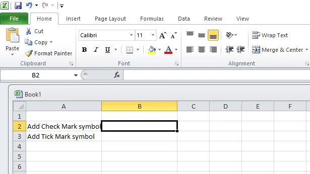
Step 1:

Select the cell in which you want to insert a check mark.

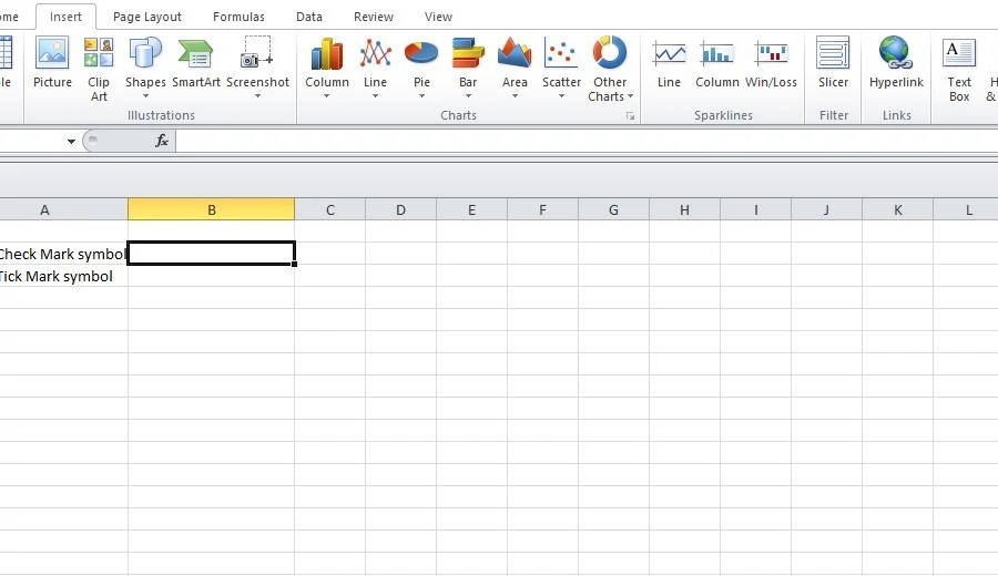
Step 2:

Go to the insert tab then select the symbol option as shown below:

Step 3:

When you click on the Symbol Option You will get the following window:

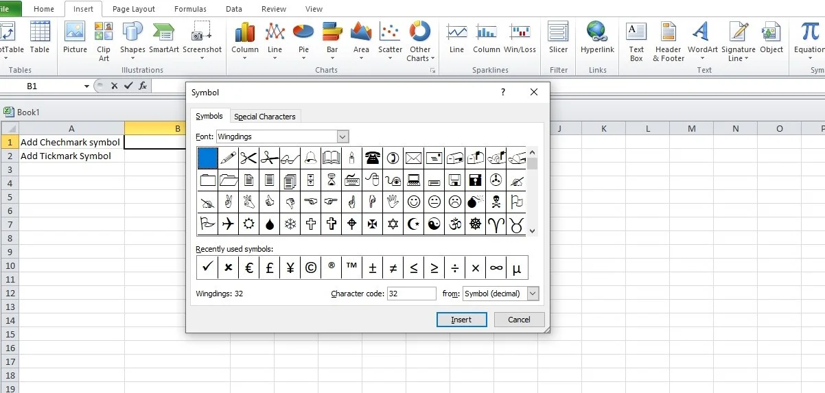
Step 4:

Now on the window select Wingdings font on the font dropdown. And in the character code box enter 252. When you enter this you will see a check mark symbol highlighted on your window.

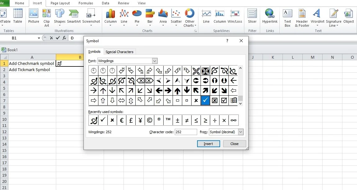
Step 5:

Now click on the insert button and then close the window. When you do this your check mark symbol will be inserted in your selected cell as:

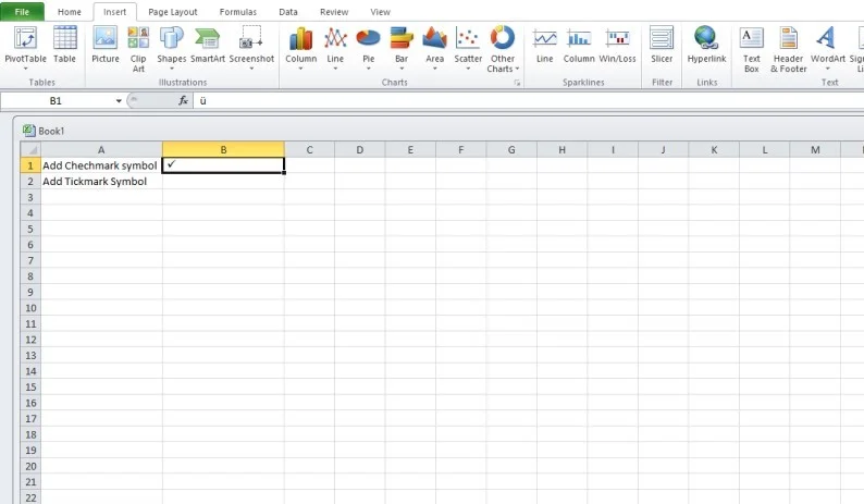
By following these easy steps you can insert a check mark symbol in your Excel spreadsheet by using the symbol command.

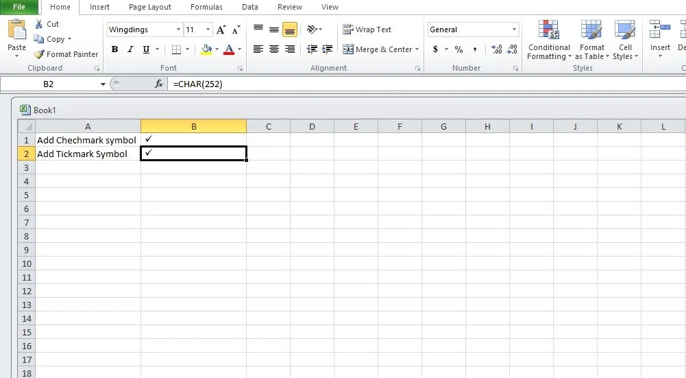
Method 2: How to Insert a Check Mark in Excel using Formulas?

To insert a check mark using this formula first of all change the font style into wingdings. Now select the cell and enter this formula as =CHAR(252) as shown below:

Method 3: Add a tick symbol by typing a character code

Another method to insert check marks in Excel is to use a character code. These are simple steps to follow to insert a tick mark in Excel using character code.

• Select the cell where you want to insert the tick mark.
• On the home tab change the font into wingdings.
• Press and hold the Alt key while writing character code 0252 on a numeric pad for the tick symbol.

        Alt +0252=tick symbol

Method 4: How to do a tick in Excel using keyboard shortcuts?

To insert a check mark using this keyboard shortcut you have to change the font style of your Excel spreadsheet to Wingding2. After changing the font style select the cell where you want to insert the check mark symbol and press Shift+P. your check mark will be added to the cell.

Method 5: How to Make a Checkmark in Excel with Autocorrect?

Excel has a feature where it can autocorrect the misspelled word automatically. For example, type the back in Excel and click enter to see what happens. Excel will automatically change this word to back. This happens when there is a pre-made list of misspelled words in Excel. When you type that word Excel will autocorrect it.

Here are some steps to insert a checkmark using the autocorrect feature.

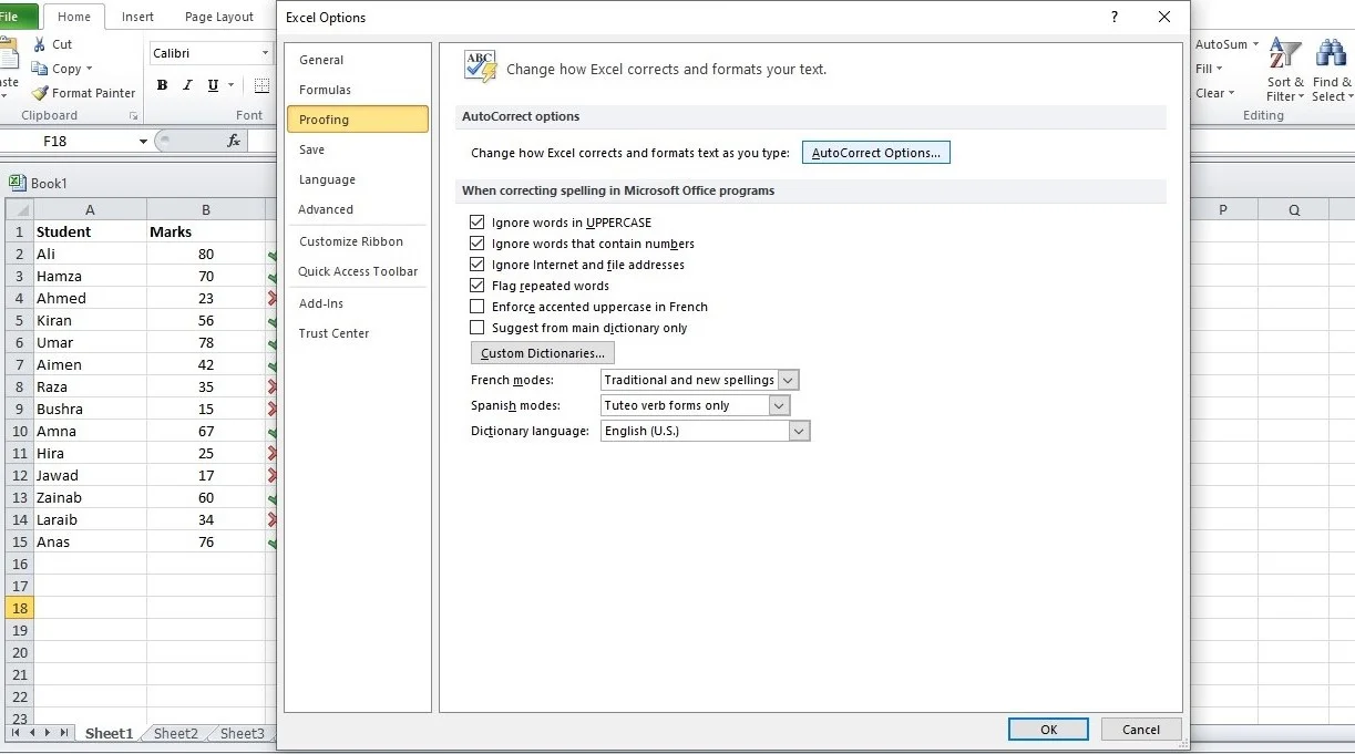
1. Click on File and choose Options.

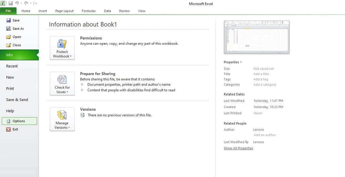
2. In the options dialog box click on proofing and select autocorrect options.

3. In the autocorrect dialog box enter the following:

• Replace: Cmark
• With: ✓(you can copy and paste this tick symbol from anywhere)

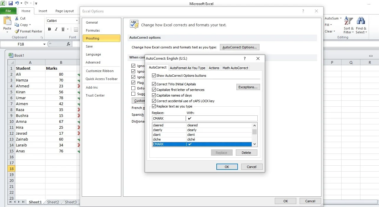
4. Click Add and the OK.

Now whenever you type CMARK in Excel it will be replaced by a Tick mark.

Method 6: Insert a Tick as an Image

One of the shortcuts to insert a checkmark in an Excel spreadsheet is simply copying the check mark symbol from Google and pasting it into the required cell. As you are reading this article you can copy this check mark and paste it in your Excel cell. Using

Method 7: Conditional Formatting to Insert Check Mark

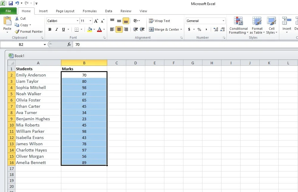
You can use Conditional Formatting to insert check marks based on the cell value. Suppose you have marks of a student between 10 to 90 and you want to mark tick for marks that are greater than 40 and cross for numbers that are smaller than 40.

Here are some easy steps to use conditional formatting to insert check marks.

1. In the cell C2, enter =B2 and then copy the formula for all cells. It will create the same value in an adjacent cell and if you want to change the value in column B it will automatically change values in column C.

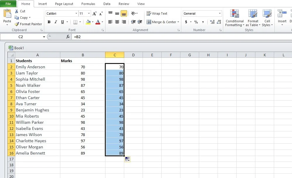
1. Select the cells in column C where you want to insert the check mark.
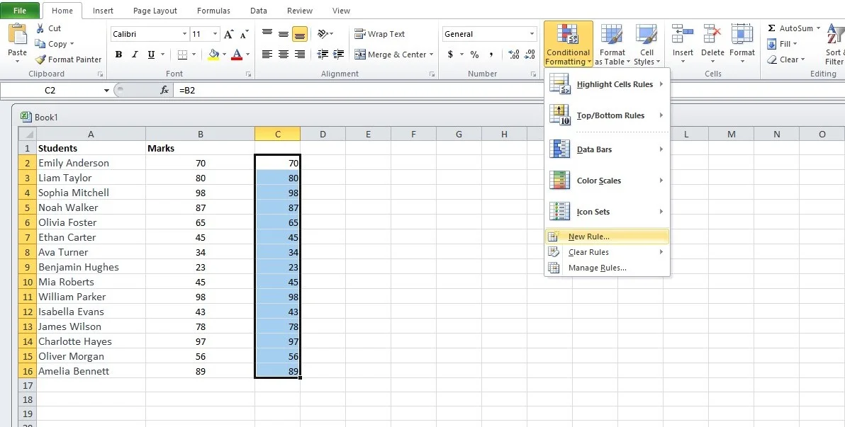
2. On the home tab click on Conditional Formatting and then select New Rule as:

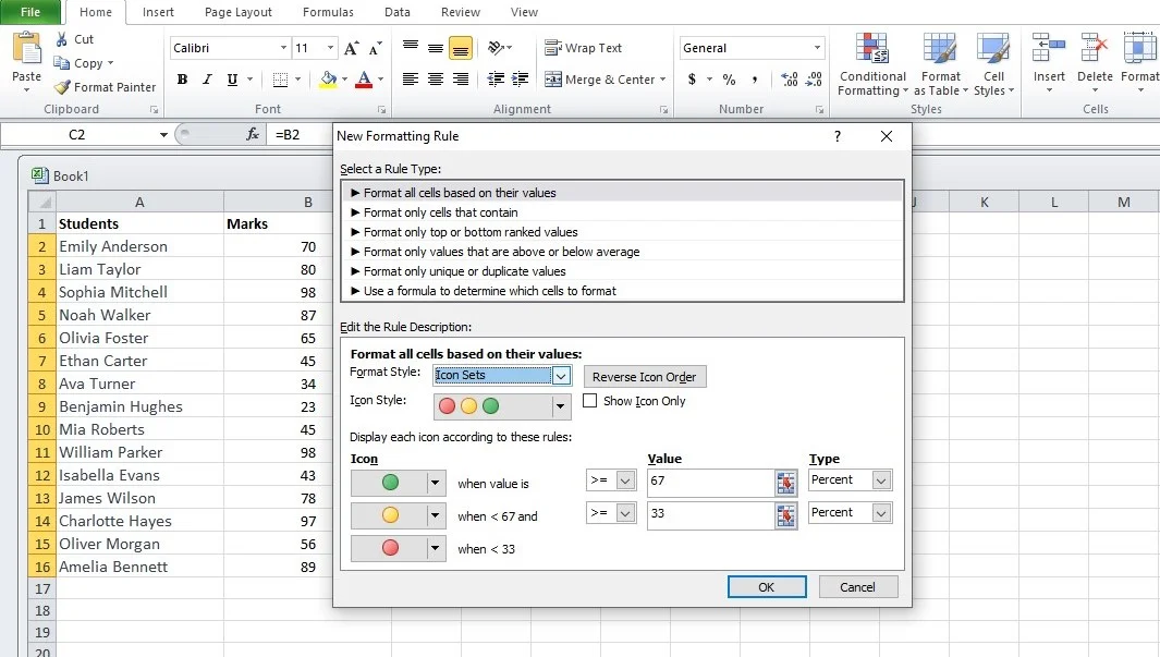
1. In the New Formatting Rule, dialog box click on the Format style drop-down and select icon sets.

1. In the icon style drop-down, select the style with a check mark and cross mark.

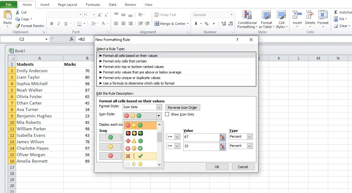
1. Check the show icon-only box. This will ensure that only icons are visible and numbers are hidden.

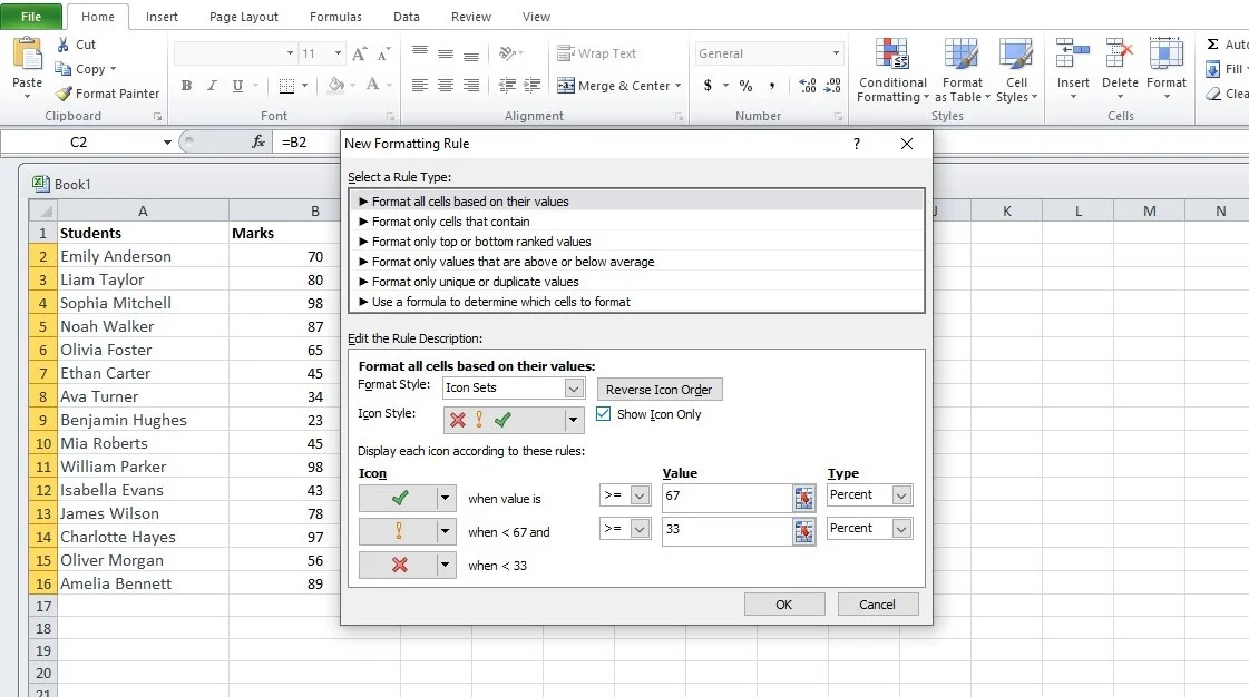
1. In the Icon setting change the percent into a number and make the following setting:

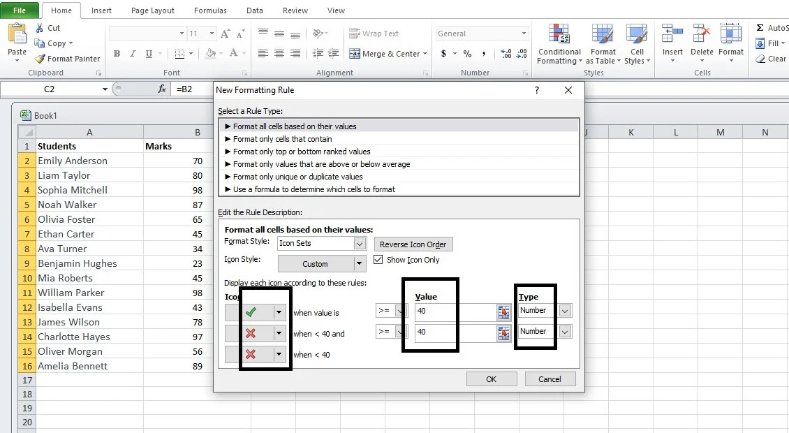
1. Click OK.
2. This will mark a green check mark for values greater than 40 and a Red Cross mark for values less than 40.

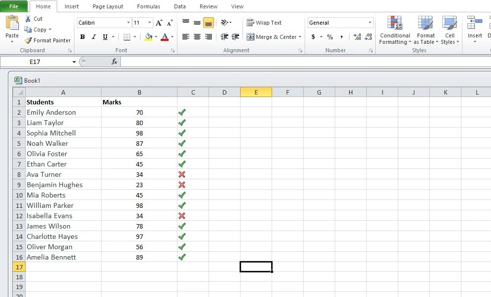
In this way, you can insert check marks in Excel using Conditional Formatting.

Method 8: Using a Double-Click (uses VBA):

With a touch of VBA code, you can implement a fantastic feature: when you double-click on a cell, it will automatically insert a checkmark, and with another double-click, it will swiftly remove the checkmark.

To achieve this, you’ll be utilizing the VBA double-click event in conjunction with a straightforward VBA code.

Before providing the complete code to enable double-click functionality, let me briefly elucidate how VBA is capable of inserting a checkmark. The following code snippet serves to insert a checkmark into cell A1 and switches the font to Wingdings to ensure that the check symbol is displayed correctly.

CODE

Sub InsertCheckMark()

Range(“A1”).Font.Name = “Wingdings”

Range(“A1”).Value = “ü”

End Sub

I will now apply the same concept to add a checkmark with a double click.

Here’s the code for achieving this:

Private Sub Worksheet_BeforeDoubleClick(ByVal Target As Range, Cancel As Boolean)

If Target.Column = 2 Then

Cancel = True

Target.Font.Name = “Wingdings”

If Target.Value = “” Then

Target.Value = “ü”

Else

Target.Value = “”

End If

End If

End Sub

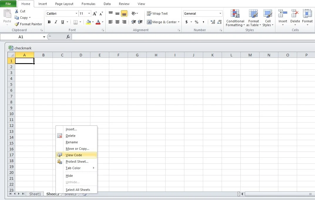
To enable this functionality, you must copy and paste the code into the code window of the worksheet where you want it to operate. To access the worksheet code window, simply left-click on the sheet name in the tabs and then select ‘View Code’.

Excel Tick Symbol – Tips and Tricks

Now you have learned how to insert the tick symbol in Excel. You may apply Formatting to it. You can count it as well.

How to format check Symbols in Excel?

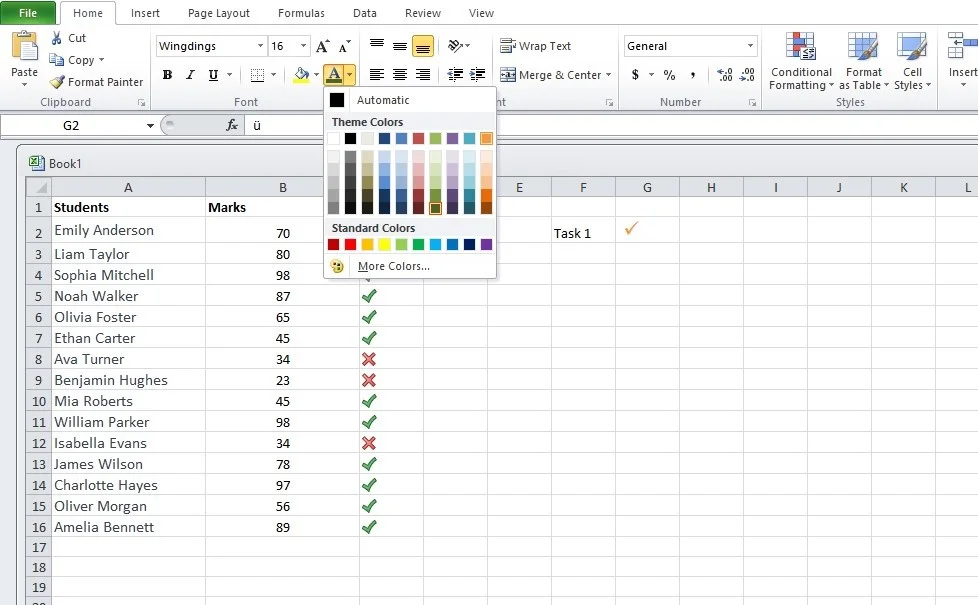
Once you have inserted the check mark in Excel it will behave like any other text. You can select the cell and format it according to you. For example, you can make it bold and you can change its color.

Conditionally format cells based on a check symbol

“If the cells in question exclusively contain a checkmark and no other data, you can establish a conditional formatting rule that will automatically apply your desired formatting to these cells. One significant advantage of adopting this method is that you won’t need to manually reformat the cells after removing a checkmark.

To set up a conditional formatting rule, follow these steps:

1. Highlight the cells you wish to format (for instance, B2:B7 in this example).
2. Navigate to the Home tab > Styles group, and click on Conditional Formatting > New Rule…
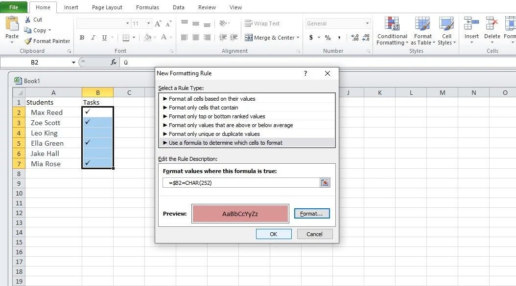
3. In the New Formatting Rule dialog box, choose ‘Use a formula to determine which cells to format.’
4. in the ‘Format values where this formula is true’ field input the CHAR formula:

=$B2=CHAR(252)

Here, B2 represents the uppermost cell that might contain a checkmark, and 252 corresponds to the character code for the checkmark symbol inserted in your worksheet.

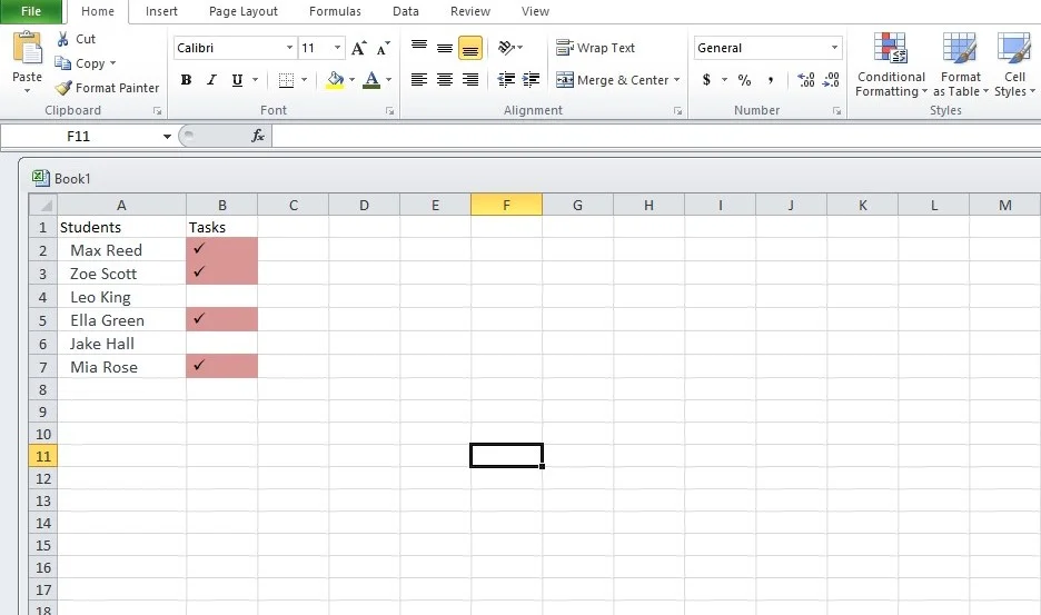
5. Click the Format button, select your preferred formatting style, and click OK.
6. The outcome will resemble something like this:”

It will be shown as this:

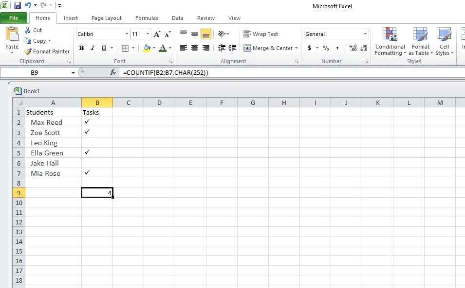
How to count check symbols in Excel?

If you want to count the total number of check marks in Excel you can do it using a combination of COUNTIF and CHAR Formula. Use the following formula

=COUNTIF(range,CHAR(252))

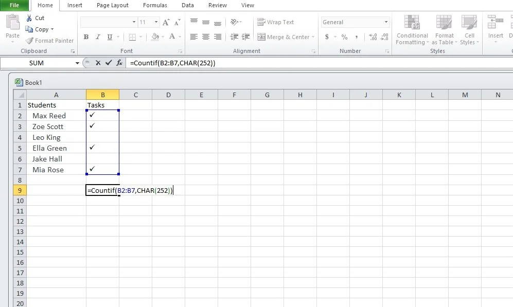
Click the Enter key.

Conclusion:

Throughout this blog, we’ve explored several methods to insert check marks in Excel, including using the Symbol command, formulas, character codes, keyboard shortcuts, autocorrect features, and even the power of Conditional Formatting. Additionally, we’ve delved into the world of VBA, where you can create a double-click functionality to effortlessly insert and remove check marks.

Related Articles:

• Insert Checkbox in Excel

Nadeem Salam

With over two decades of experience in writing about Microsoft Excel, Google Sheets, and various other spreadsheet tools, Muhammad Nadeem Salam is your go-to expert for all things data. Since 2004, he has been passionately sharing his knowledge and insights through engaging and informative blog posts, helping countless readers unlock the full potential of their spreadsheet tools.