Excel is an essential tool for professionals worldwide in the ever-evolving field of data management. One activity is identical regardless of data analysis skill or where you are in your data journey: comparing two columns.
For example, if you have so much data and want to fill the spreadsheet, your goal is to find the same values in two columns. It may look difficult, but don’t worry! We are here for you to guide you.
In this article, we explain how to compare two columns in Excel step-by-step, equipping you with the methods and strategies necessary to speed up your data analysis workflow.
What Do You Mean by Comparing Columns in Excel?
Excel makes it easy to compare columns by comparing each cell to the target cells to see if they match and, if not, show a suitable message.
It helps locate and fix data imperfections, such as misspelled names or incorrect formatting. You can use Excel’s filtering and sorting functions to organize data based on specific criteria.
How to Compare Two Columns in Excel?
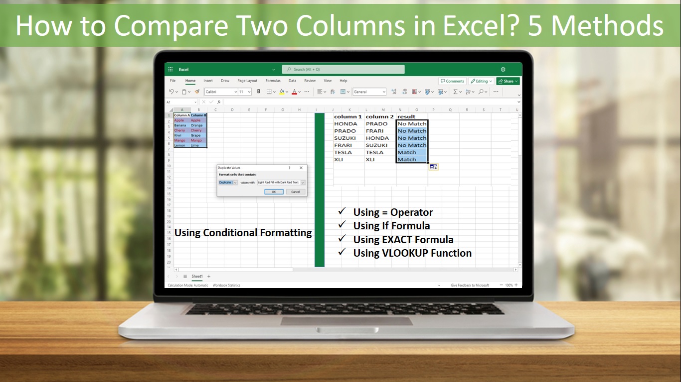
Here are some effective methods to compare two columns in Excel:
- Conditional Formatting in Excel
- Using Equals Operator
- Using VLOOKUp Function
- Using the IF Formula
- Using the EXACT Formula
Method 1: Conditional Formatting in Excel
Excel’s Conditional Formatting is one of the easiest methods for comparing columns. Here are some steps for conditional formatting in Excel:
Step 1: Select the column of the cell in the Excel sheet.
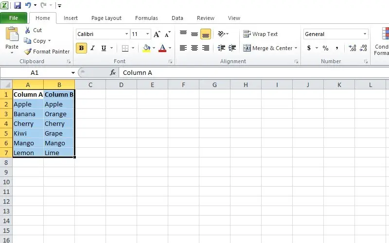
Step 2: Go to the “Home” tab. Tap on “Conditional Formatting” in the “Styles” group.
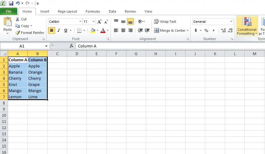
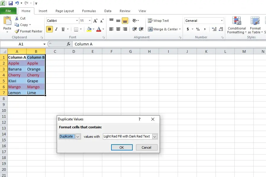
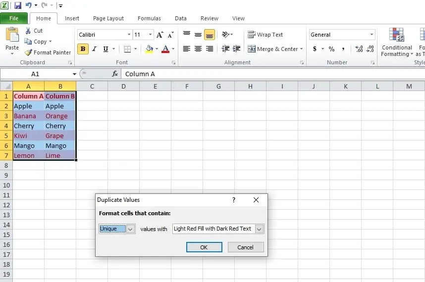
Step 3: Tap on highlight cells rules. On the screen, a new window with options to select for “Duplicate” and “Unique” values will emerge..
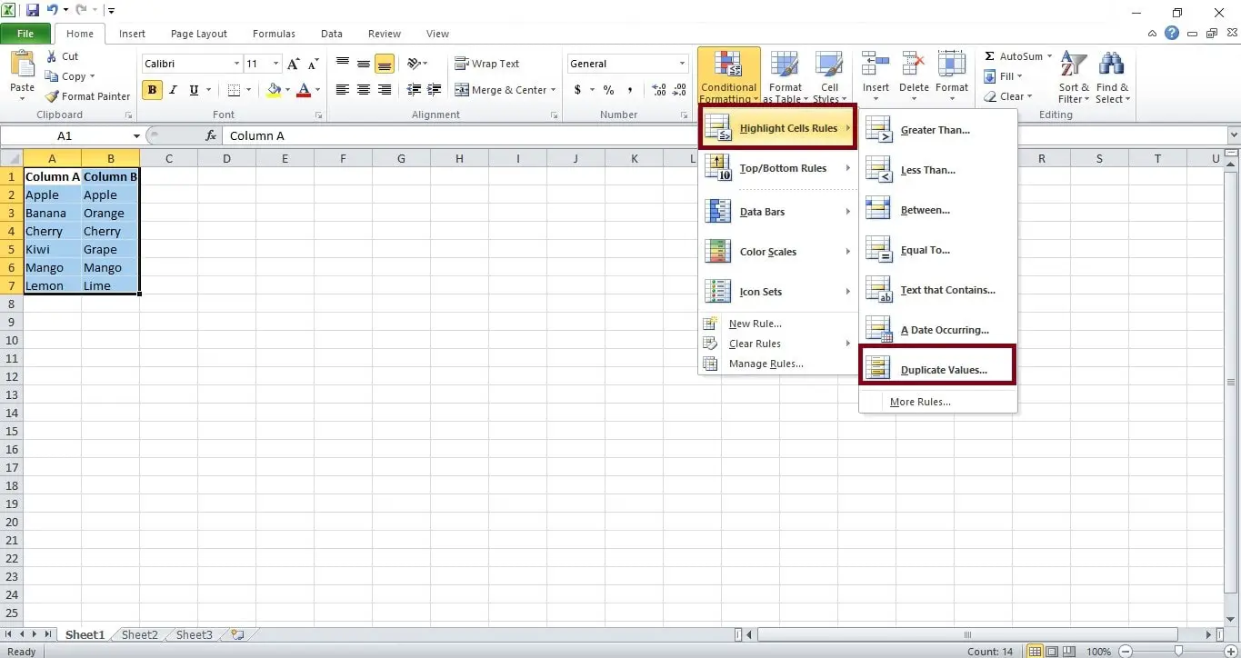
Step 4: Now, you can compare the two columns with matching or unique values.
Duplicate values
Unique values
Method 2: Using Equals Operator
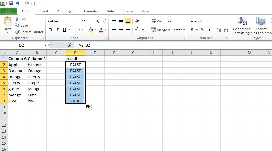
Excel’s equal operator is a further simple method for comparing columns. Here are the following steps to compare two columns in Excel using the equals operator:
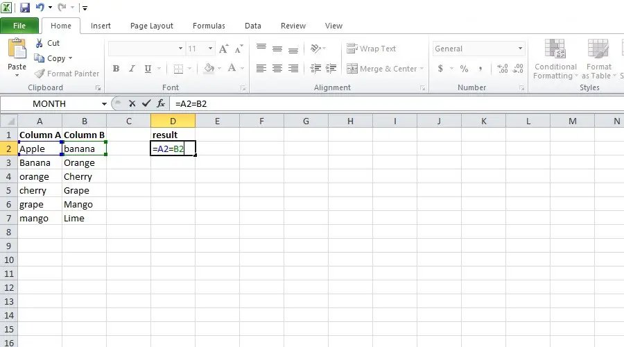
Step 1: Add the formula for individual cell comparison to a new result column. As shown below;

Step 2: For every comparison that is failed, FALSE, and for every comparison that is successful, TRUE.
Method 3: Using the VLOOKUp Function
Now we will guide you about 3rd method to compare two columns in Excel. Here are the following steps to compare two columns in Excel by using the VLOOKUP Function;
Step 1: To display the desired VLOOKUP result in the desired cell.
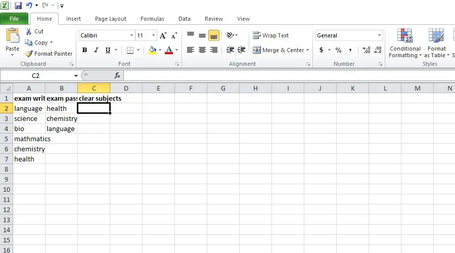
Step 2: Write a formula of VLOOKUP Function that is =VLOOKUP (lookup_value, table_array, col_index_num, [range_lookup]).
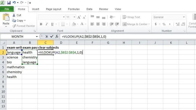
Step 3: Press enter, and the result will shown below.
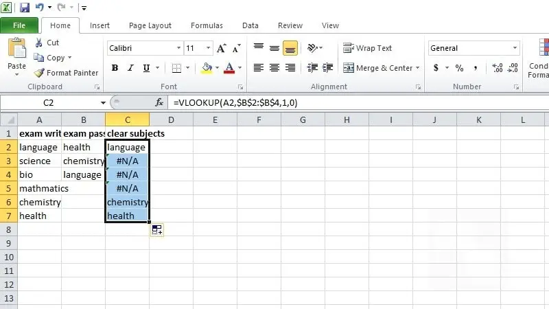
Method 4: Using the IF Formula
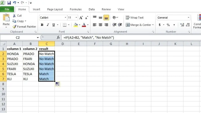
When comparing two columns in Excel, the IF formula is used to provide a desired result for a similarity or difference. Below are steps to compare two columns in Excel by using the IF formula:
IF Formula: =IF(A2=B2,”Match”, “NoMatch ”)
- Step 1: Create a new column wherever the comparison results should be displayed.
- Step 2: Type the following formula in the first cell of the new column: =IF(A1=B1, “Match,” “No Match”).
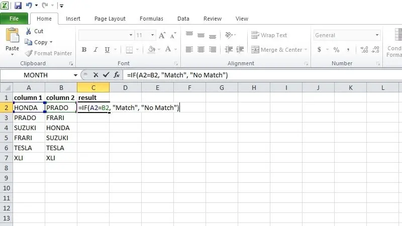
- Step 3: press “enter” and then drag the formula to all desired cells. The below table will show:
Method 5: Using the EXACT Formula
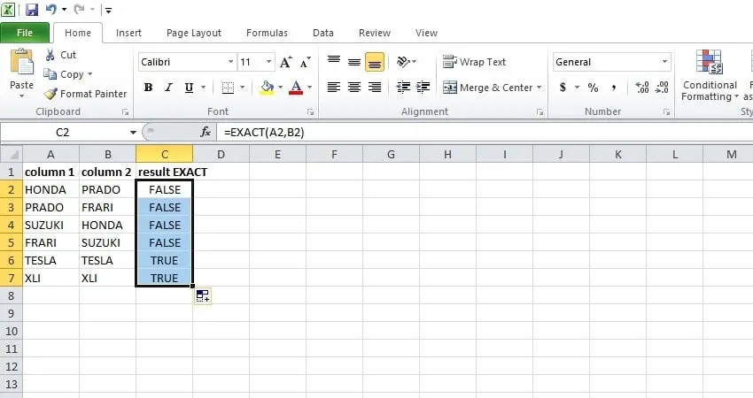
Here are steps to compare two columns in Excel by using the EXACT formula:
- Step 1: Choose a third column where you want to display the comparison results, whether column A and Column B are the same or not.
- Step 2: Tap on the cell in the third column and enter the following formula.
=EXACT(A2, B2)
- Step 3: Then press “Enter” to calculate a result.
- Step 4: Click and drag this fill handle downward to apply the formula to all rows. Moving Excel down will automatically change the cell references (A1, B1) to compare the matching cells in columns A and B.
Why Compare Two Columns in Excel?
Comparing two columns in Excel can assist you in the following way:
- Quickly find duplicates of data elements like customer names or product IDs in a dataset.
- Find data inconsistencies, such as disparities between inventory and sales records.
- Verify that two columns match to ensure data accuracy, essential for error-free reporting.
Which Method to Use in Each Scenario
Here, we provide you details of which method you will use in each scenario:
Scenario 1: Compare Two Columns in Excel Row-by-Row
In Excel to compare two columns in row-by-row, the following formulas you can use:
- =IF(A2 = B2, “match”, “ ”)
- =IF(A2<>B2, “no match”, “ ”)
- =IF(A2 = B2, “match”, “no match”)
Scenario 2: Compare Multiple Columns for Row Matches
Use the following formulas if you need to contrast and identify the differences and similarities between more than two columns:
- =IF(AND(A2=B2, A2=C2, “Complete match”, “”)
As 4 is the number of columns you are comparing, write =IF(COUNTIF($A2:$E2, $A2)=4, “Complete match,”
The following formulas can be used to compare columns if two or more cells have the same value in the same row.
- =IF(Match, “Match”, “OR(A2=B2, B2=C2, A2=C2), “”)
Scenario 3: Compare Two Columns for Matches and Differences
Any of the following formulas for determining the match and differences can be used to compare two datasets and identify the unique values that are present in column A but not in column B:
- =IF(COUNTIF($B:$B, $A2)=0, “Not present in B”, “”)
- =IF(ISERROR(MATCH($A2,$B$2:$B$10,0)),”No present in B”,””)
Scenario 4: Compare Two Lists and Pull Matching Data
You can use the VLOOKUP INDEX function to compare two lists and locate the matched data.
- =VLOOKUP(D2, $A$2:$B$6, 2, FALSE)
- =INDEX($B$2:$B$6, MATCH($D2, $A$2:$A$6, 0))
Conclusion
Everyone who works with data has to be capable of comparing two columns of data in Excel. Excel offers several features to make this process accurate and effective, whether you need to clean your data, reconcile records, or find patterns.
This article has given you in-depth details on How to compare two columns in Excel. Now, you can easily compare two columns.
FAQs:
How do you compare two columns in Excel?
To compare two columns in Excel, use the following actions: Select both data columns, pick the Home tab, and click Find & pick. Choose Go To Special. Click OK after selecting Row Differences.
Can we compare two columns in Excel using the Index-Match function?
You can use Excel’s Index-Match function to compare two columns if you create an appropriate formula for the required information.
How do I compare two columns in Excel and count matches?
Using the new column’s first cell as your entry point, type =SUMPRODUCT((A2:A=B2:B)*(C2:C)).
This formula instructs you to compare the values in columns A and B and, if they coincide, to return the value in column C.
With over two decades of experience in writing about Microsoft Excel, Google Sheets, and various other spreadsheet tools, Muhammad Nadeem Salam is your go-to expert for all things data. Since 2004, he has been passionately sharing his knowledge and insights through engaging and informative blog posts, helping countless readers unlock the full potential of their spreadsheet tools.
