Google Spreadsheets is a convenient and versatile tool for gathering, managing, and processing data. It also has many good features, like sharing with the team and data storage online, which makes it the choice of many business professionals. Pivot Table in Google Sheets is no doubt one of the best features.
Many business people, analysts, and researchers use Excel, and if you ask them why, the response will be that it has pivot tables. Do you know that Google Sheets also has Pivot tables, which you can use to summarize, filter, and process data?
If you do not know how to create & use a Pivot table in Google Sheets, then do not worry. We have created this Pivot table in the Google Sheets guide for you. This blog will tell you everything related to pivot tables in Google Sheets.
Let’s get started with the definition of Pivot tables:
What is a Pivot Table in Google Sheets?
Pivot tables are the best way to summarize large data sets in Google Sheets. We usually have data in rows and columns in Google Sheets. When working in an organization or doing a big project, you typically have an extensive data set to process.
But it’s not easy to process large data sets in Google Sheets. For this, we need Pivot tables. The pivot table helps you to distill the information in that large dataset. Pivot tables also allow you to filter the data based on different variables in the data.
You do not always have to create reports from scratch. As you can use pivot tables to create different reports in a few clicks. If you get extra rows in your data, just change the range of pivot tables. Your report will be updated.
Uses of Pivot tables:
Here are some uses of the Pivot table in Google Sheets
- Pivot tables help you filter large data sets.
- Pivot tables give you a more focused image of your data.
- Pivot table enables you to create reports on data in a few clicks.
- The pivot table helps you analyze the data and find actionable insights.
- The pivot table summarizes the data and shows you totals, averages, and other calculations on clicks.
How to Create & Use Pivot Table in Google Sheets?
Pivot tables are effortless to use in Google Sheets. By manually creating a pivot table in Google Sheets, you can select which variables should go in rows and which should go in columns. Which columns to use as values? You can also choose variables/columns in data to work as a filter in Google Sheets.
Creating Pivot Table in Google Sheets
Let’s get started with pivot tables in Google Sheets. Follow the steps below to create pivot tables.
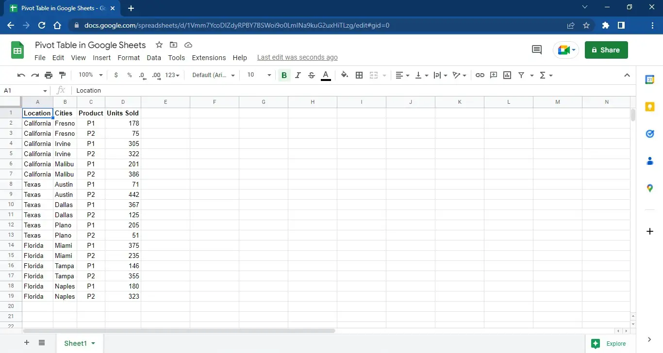
- Open your Google Spreadsheet.
- Enter the data on which you want to do the analysis.
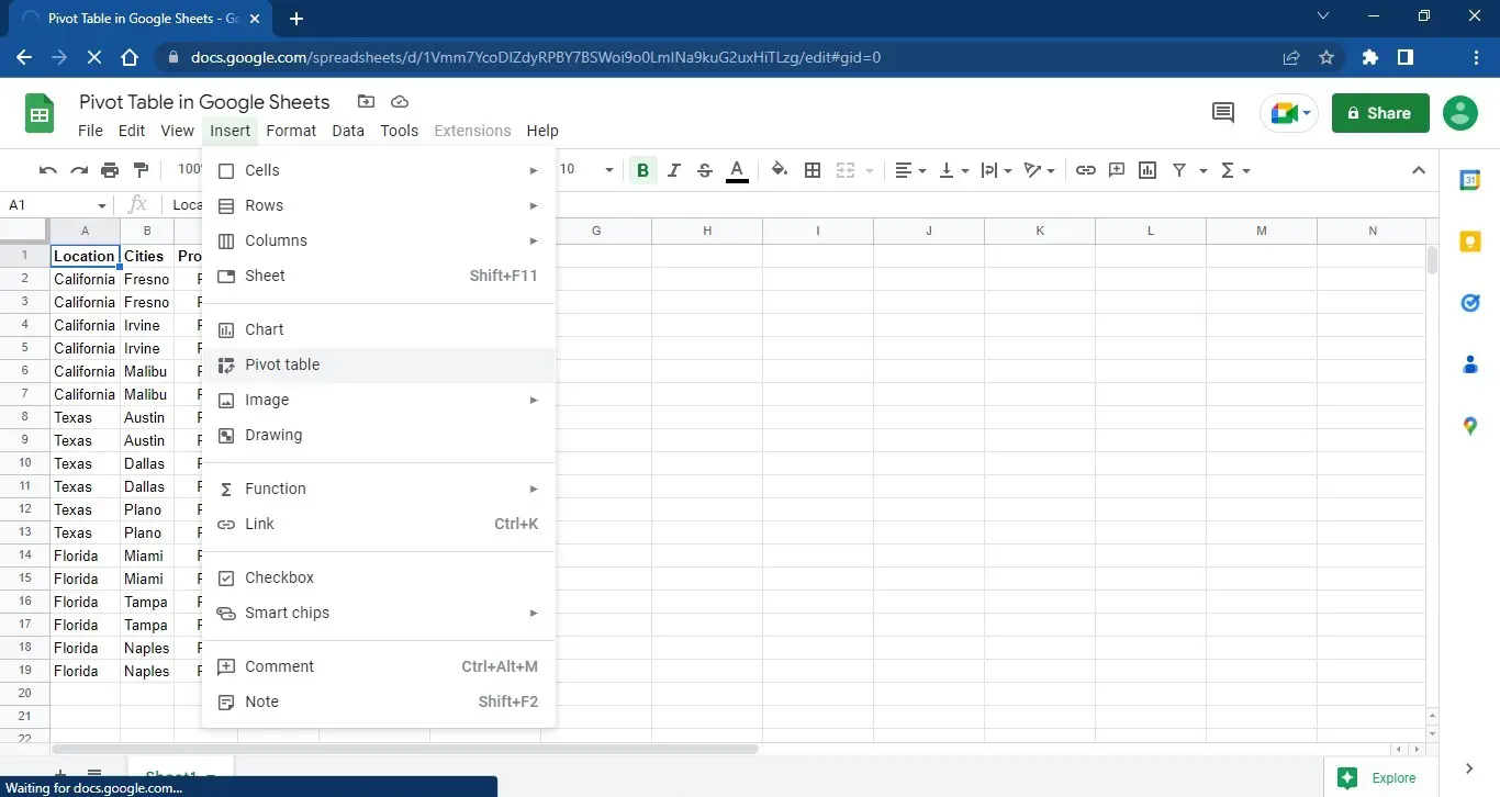
- Next, go to Menu and find the “Data” tab in it.
- Click on “Insert” to see “Pivot table” in the drop-down list, as shown below.
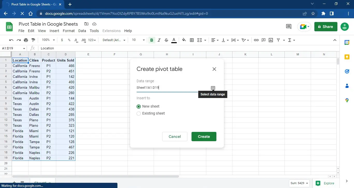
- Now select the data range on which you want to create a pivot table.
- After selecting data, you need to choose whether you want to create a pivot table on an existing sheet or create a new one. You can select either option, whichever suits you best. In our case, we will go with the “new sheet”.
- The following screen will show once Google Sheet has created a pivot table for you, as shown below.
- Google Sheets will name this sheet automatically on the pattern of Pivot Table 1, Pivot Table 2, and so on.
Using Pivot Table in Google Sheets
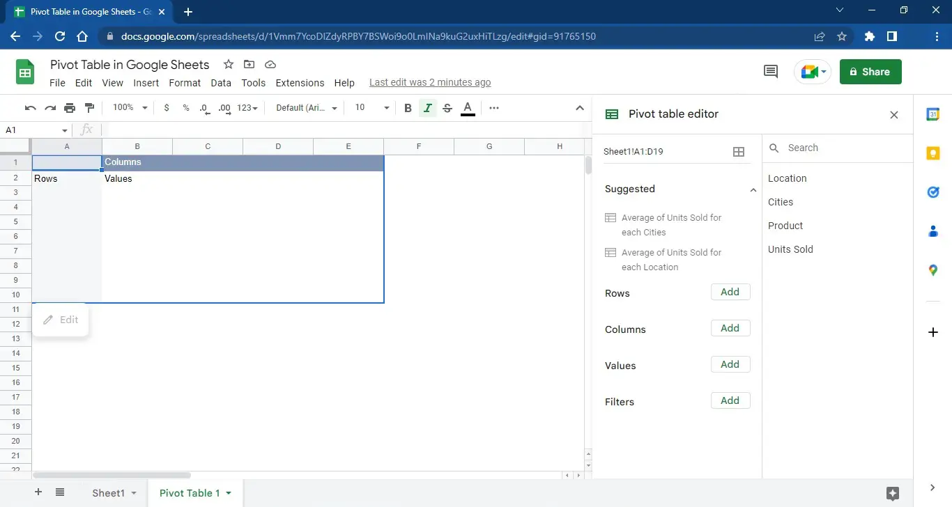
- Next, tell Google Sheets what you want to be in Rows, Columns, Values, and Filters.
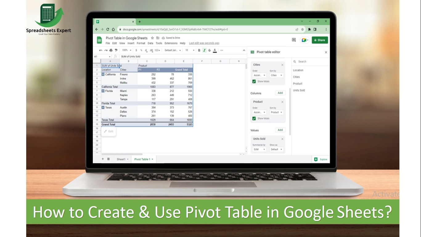
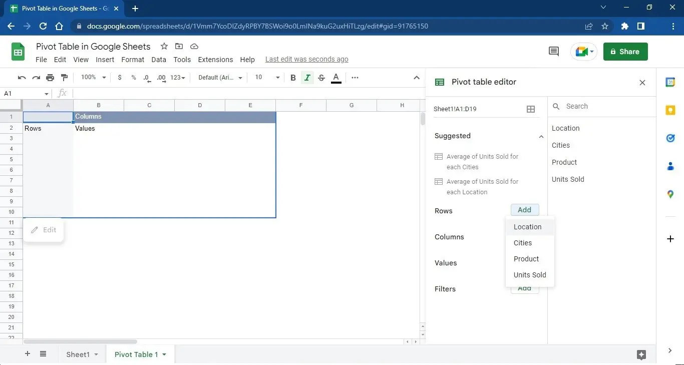
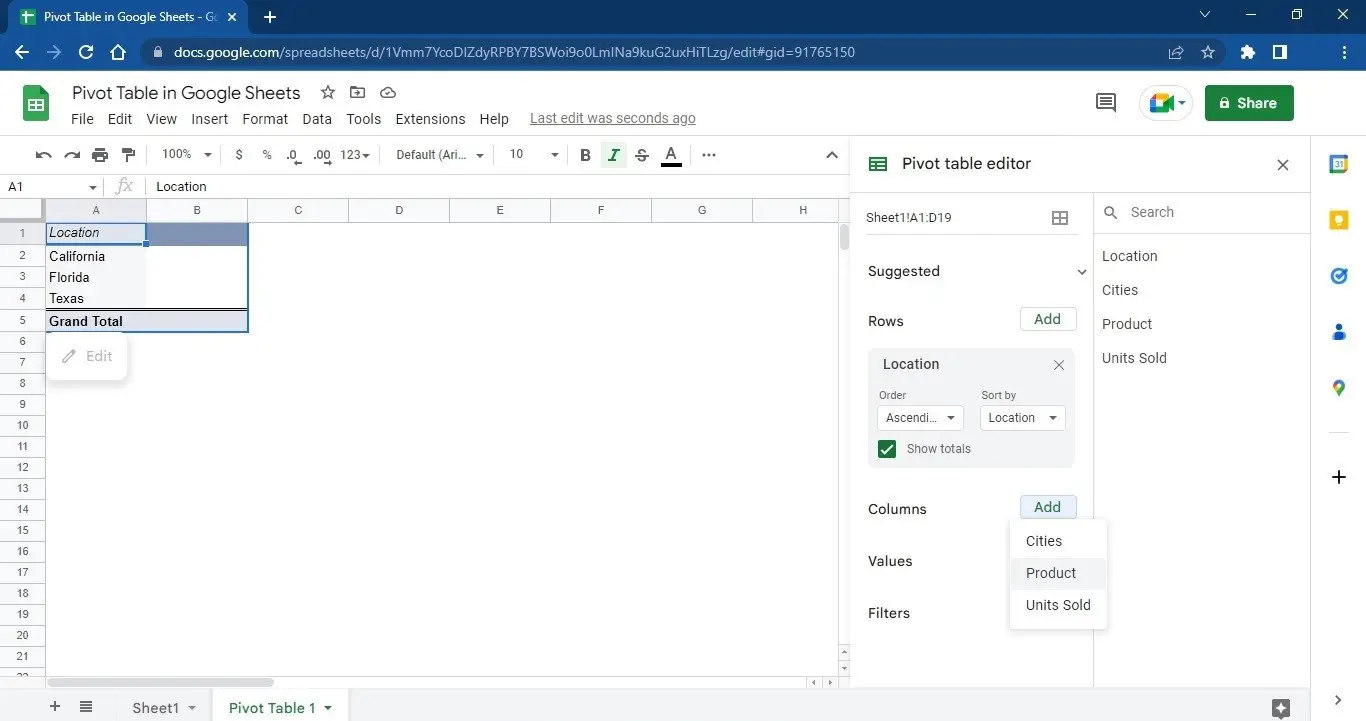
- In our case, we will select Location for Rows, as shown below.
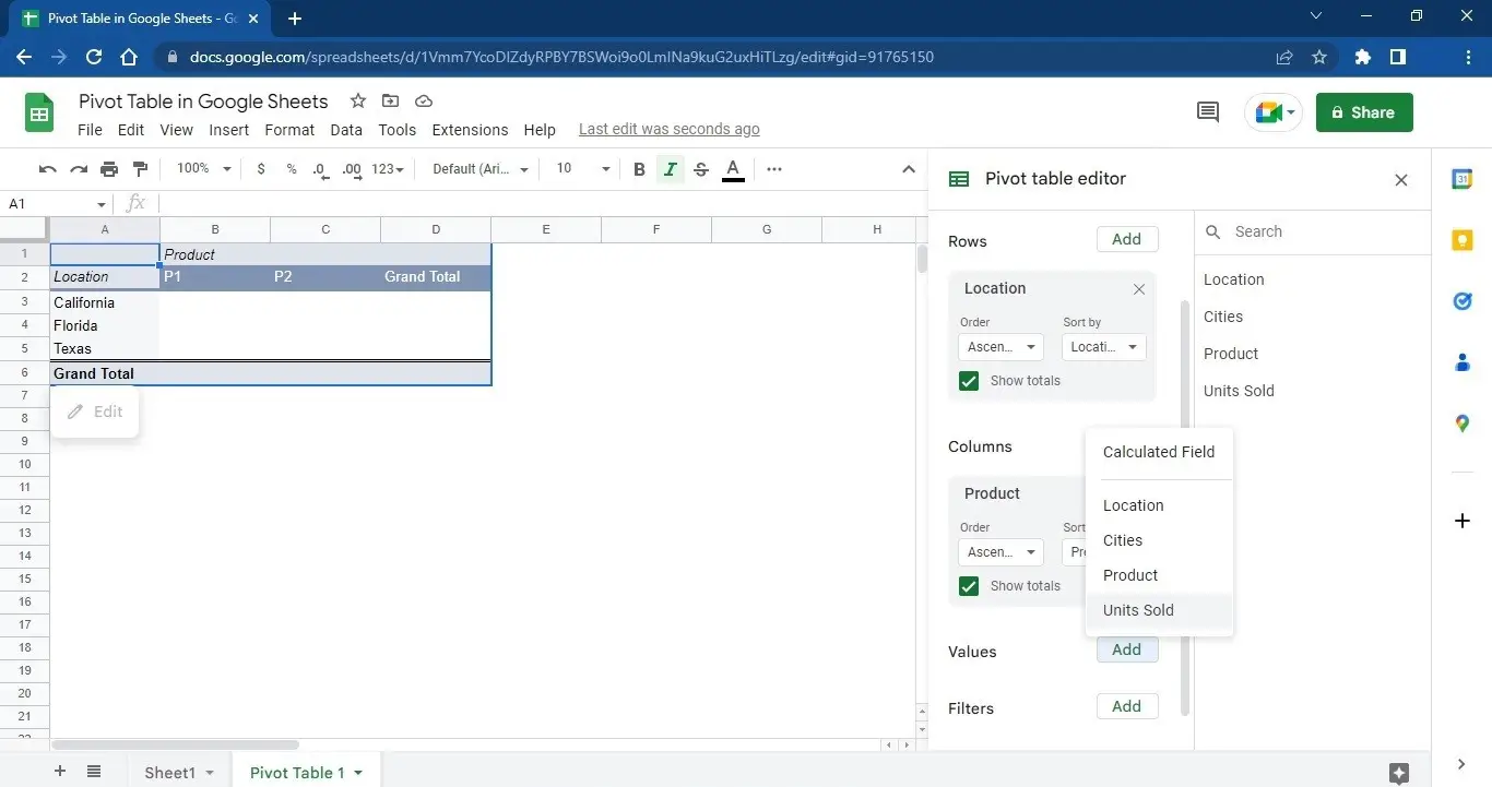
- After Selecting the Rows, the Next thing to select is a Column. We will choose Products in Columns, as shown below.
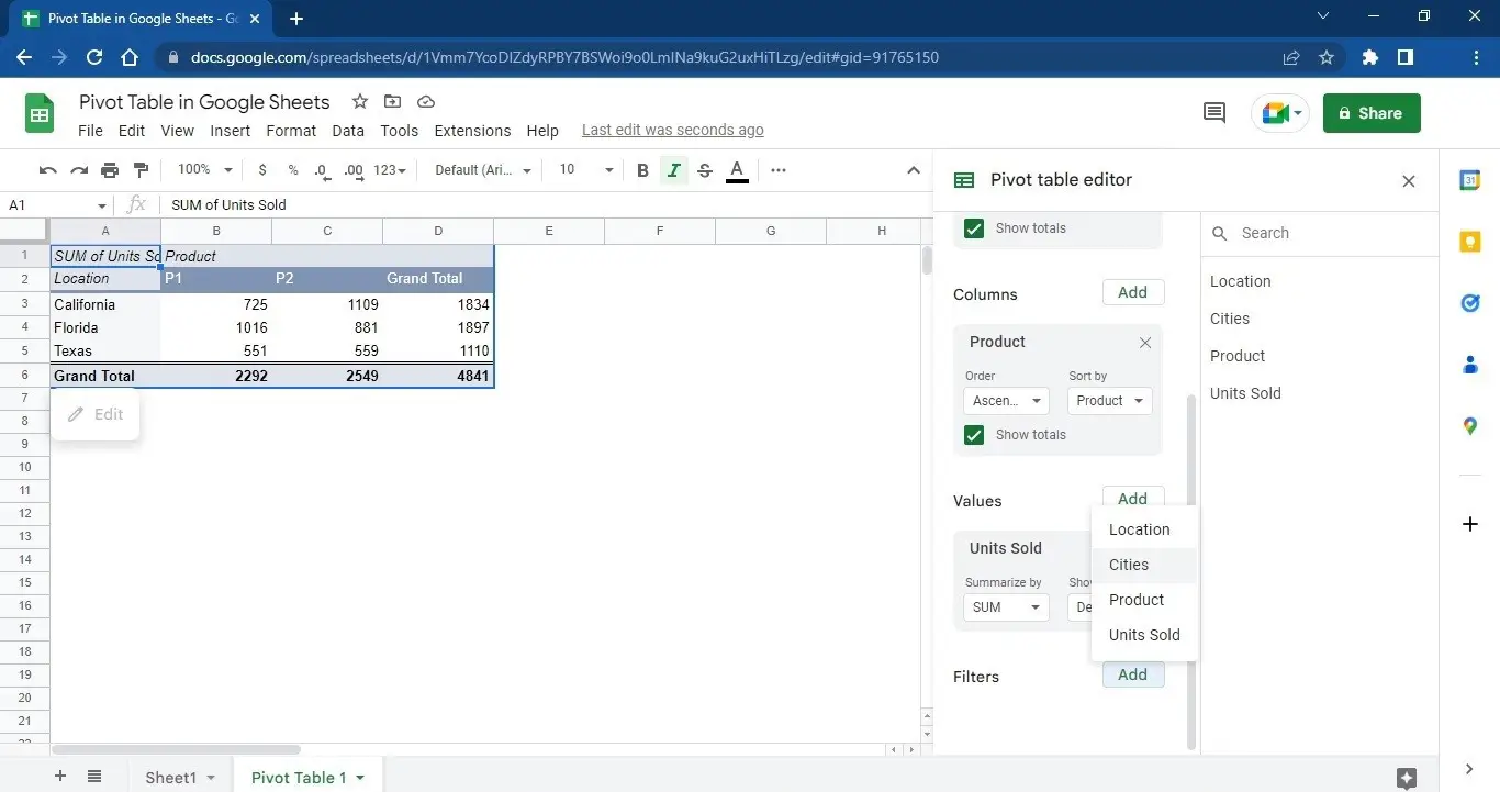
- Now, we have selected Rows and columns. Then, the next thing to tell the Pivot Table is Values. This means which column to take as values. In this example, we will select Units Sold as Values.
- If you want to apply any filter, select that column in Filter. You can choose already selected columns or unused columns. Let us show how to do it by selecting Cities in Filter.
- You can also select multiple columns in Rows, Columns, Values, and Filters. Let us show you how you can use it.
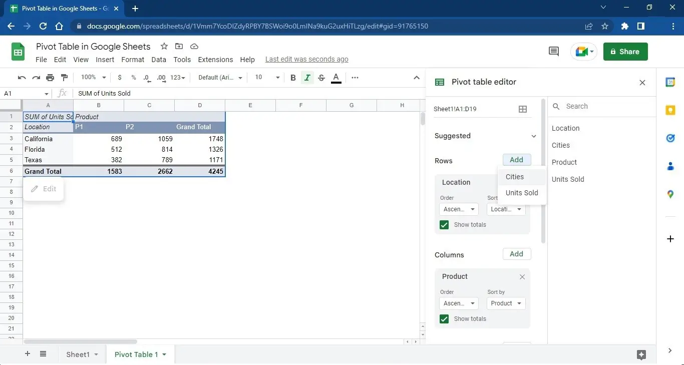
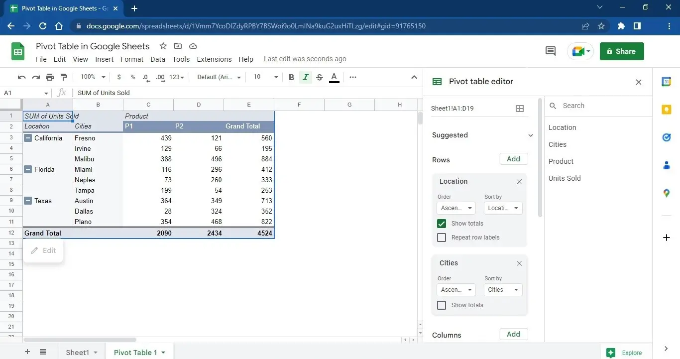
- Click on Add in front of Rows to add Cities in rows. Results will be as follows after the selection.
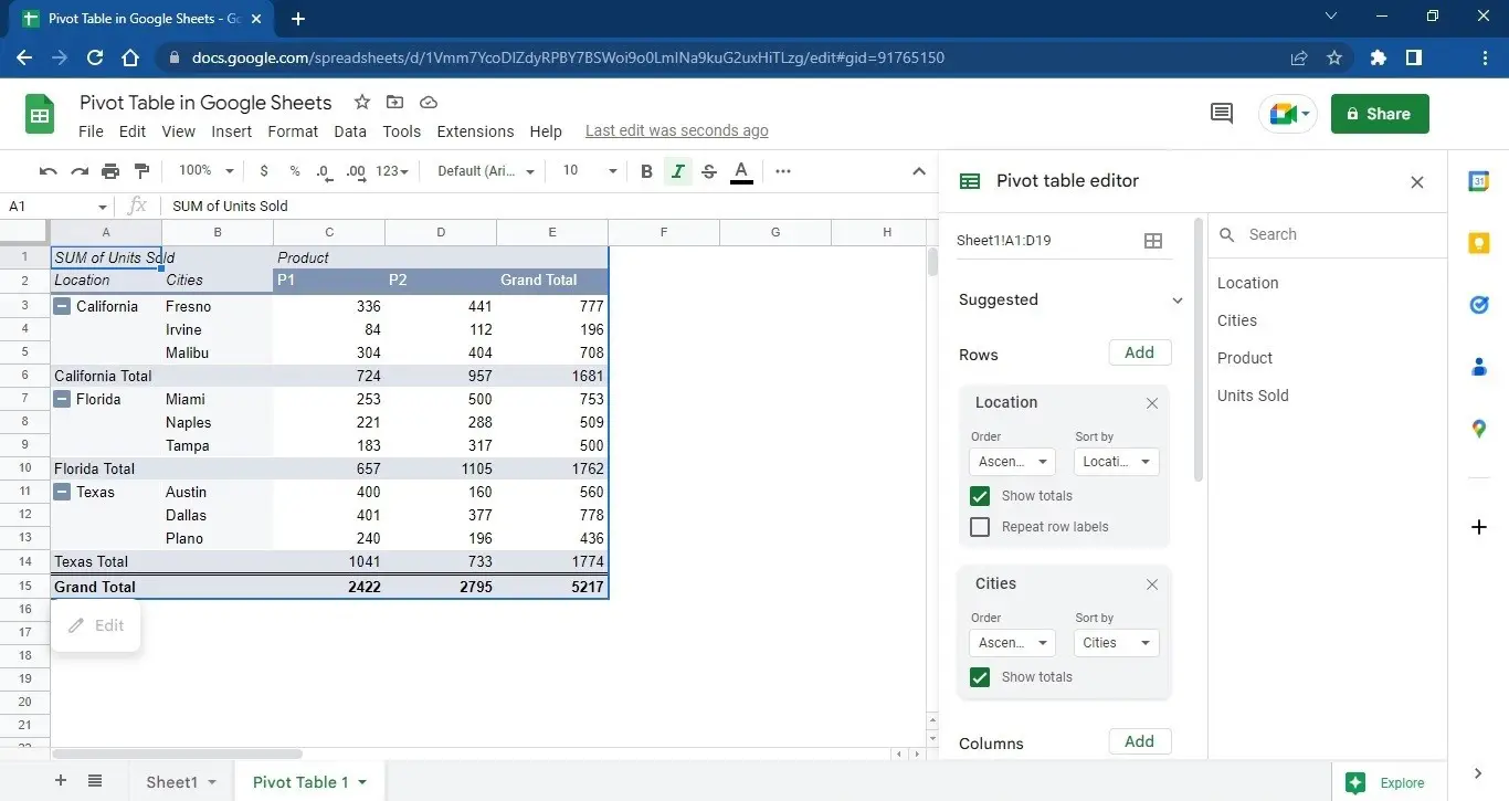
- The image above shows the final Pivot Table we created on our data set. You can follow the steps mentioned above to start a Pivot Table on any of your datasets. Pivot Tables will help you summarize and filter the data to analyze it and extract actionable insights.
How to Show Total Rows in Pivot Table?
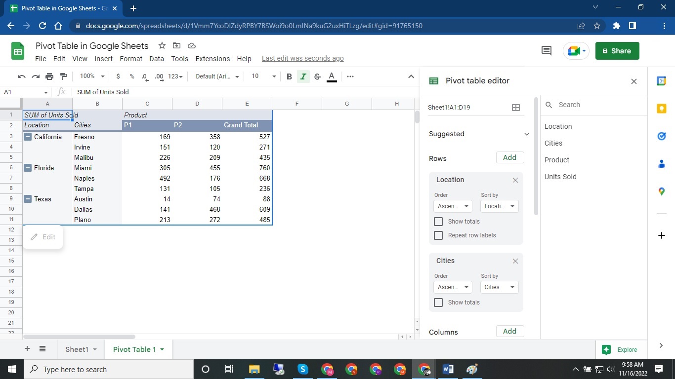
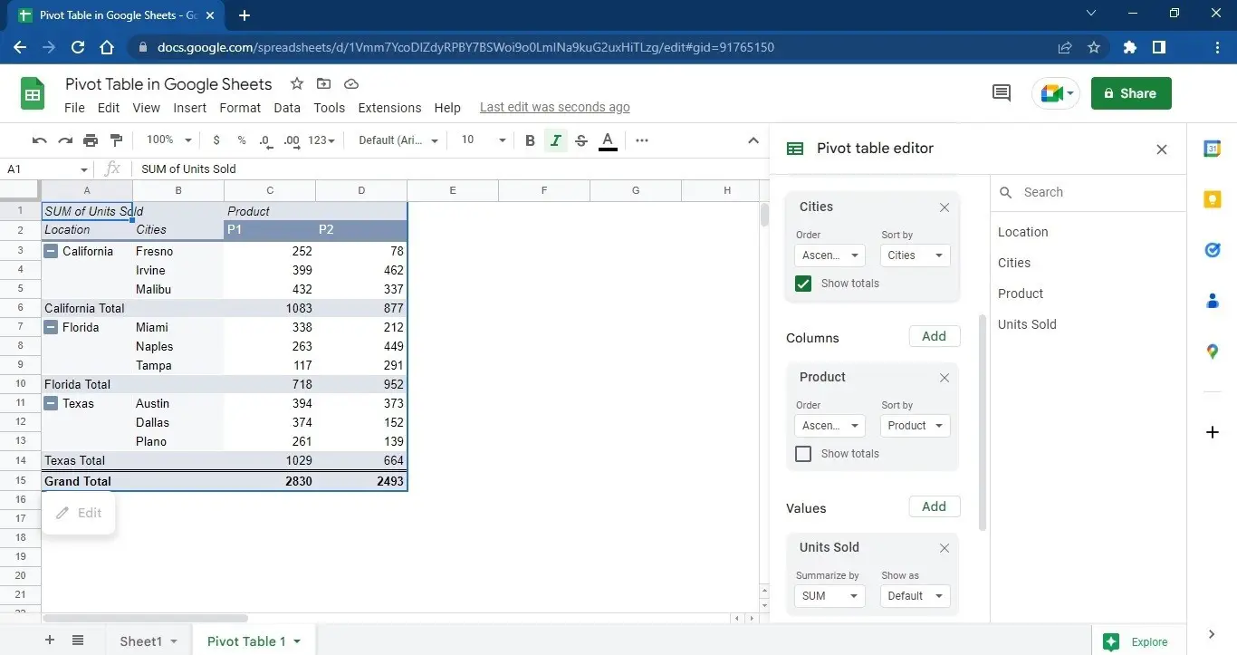
It’s straightforward to show the Total of values against rows. E.g. In our example, if the “Show Totals” checkbox is unchecked, then the results will look like as below:
If you check “Show Totals,” the Pivot table will show you the sum against each record in a row, as shown below.
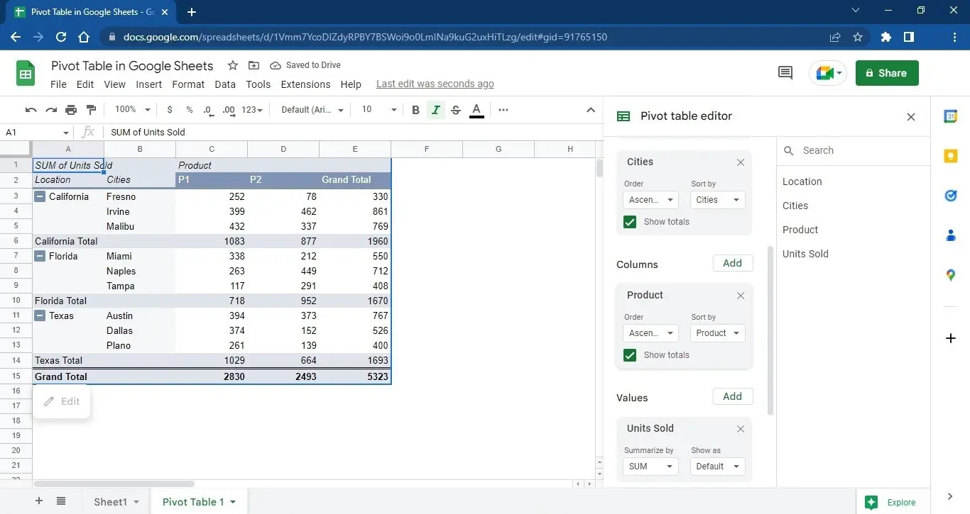
How to Show Total Column in Pivot Table?
Without showing the total column, the Pivot Table looks as follows:
- To show the Total Column, check the “Show Totals” in the Columns sections of the Pivot Table editor, as shown below:
With over two decades of experience in writing about Microsoft Excel, Google Sheets, and various other spreadsheet tools, Muhammad Nadeem Salam is your go-to expert for all things data. Since 2004, he has been passionately sharing his knowledge and insights through engaging and informative blog posts, helping countless readers unlock the full potential of their spreadsheet tools.